Reference

Complex arguments

Some of the function arguments expect certain types of values that can't be shortly described. Therefore, they are referenced in the documentation below by their unique names, whereas simple arguments have an in-line description. The description for such complex arguments is provided below.

Index

is a list of values in square brackets, separated by commas or colons. Each value can be either a number or a string. Colons are used to specify a range of values, e.g. [1:4] is equivalent to [1, 2, 3, 4]. For string values it's also possible to specify an offset: ["Total"(+2)]. The offset value can be either positive (+2) or negative (-1), which allows us to reference a row/column that goes after or before the anchor "Total".

Axis

defines whether to apply an operation on rows or columns. Use 0 or "rows" for rows and 1 or "columns" to apply to columns.

DataFrame

is a table of values. All expressions result in a dataframe. So when you see that the expected argument type is DataFrame, it means that the argument must be an expression. An expression can be as simple as a single SELECT or it can be a complex chain of operations.

In our examples a data frame can be represented as a 2D array. A 3x3 dataframe would look like this: [[x0, x1, x2], [x3, x4, x5], [x6, x7, x8]].

Condition

primarily used for FILTER. It expects a short comparison expression that has an arbitrary variable name on the left, a comparator in the middle (>, <, ==, <=, >=), and a string/number on the right. Something like this: x > 25.

Operations

Here is a list of all available operations that can be used to select, transform and join dataframes.

SELECT

Select data from an available data source.

Parameters:

Name	Type	Description	Default
`file`	`int \| str`	the number or the name of the attached data file.	`1`
`table`	`int \| str`	the number or the name of the table in the file.	`1`
`sheet`	`int`	the number of the sheet in the file	`1`
`rows`	`Index`	table rows to be selected.	`[:]`
`columns`	`Index`	table columns to be selected.	`[:]`

Raises:

Type	Description
`IndexError`	when the specified rows/columns aren't present in the dataframe.

Usage

SELECT(file=1, sheet=1, table=2, rows=[1], columns=[2])

or a short version:

S(f=1, s=1, t=2, r=[1], c=[2])

Remarks

The table argument works with table names only if the table name location was previously specfied in the UPLOAD query. Otherwise, it won't know how to identify a table by its name and throw an error.

The sheet argument will be able to pull from sheets that have been identified in the UPLOAD query. SELECT only cares about the sheets that have been identified in UPLOAD and not any unchosen sheets from the oringinal data. For example, my UPLOAD query could be: UPLOAD (name="data", sheet=[2, 5, 7]) This would upload the 2nd, 5th and 7th sheets from my data file. However, the sheet argument in a SELECT query for this data could only be 1, 2 or 3, which would grab the 2nd, 5th or 7th sheet respectively.

An argument for columns or rows is an array (square brackets) of individual values (literals or variables) or ranges. Values must be separated by commas. For instance: [f=1, t="Total", r=[4:8], c=[1, 5, 7]. Index values are called indexers.

A range may have up to 3 explicit parameters: start, stop and step. The last parameter allows us to step over every 2nd/3rd/etc value in the range.

Examples: 1. : - full range; 2. 2: - from the 2nd to the end; 3. "Total":-2 - from "Total" to the end but 2; 4. 1:10:2 - odd ones from 1 to 10; 5. -1::-1 - full range in the reversed order;

Indexing with string literals has additional features: wildcard and relative offset. Wildcard allows to reference cells with just parts of their full values. For instance, instead of I am a disgustingly long string to type it's possible to just use *disgusting* instead. The first occurence that matches the pattern will be used.

Relative offset allows to reference rows/columns that sit next to some "anchors", i.e. rows/columns that are easy for us to find and use. Example: "Base"(+1), "Mean"(-2).

The rows and columns arguments not only dictate which rows/columns to include in the data set, but also in what order. Thus, columns=[3, 2, 1] gives columns 1, 2, 3 in the reversed order.

Example

SELECT (f=1, t=1, rows=[3:8], columns=["Total":"Female"]) >> (1, 1)

all positional arguments, this will select all columns between the column named Total and the column named Female.

SELECT (rows=[3:8], columns=["Total*"]) >> (1, 1)

only keyword arguments (use default values for the rest), this will select the first column that starts with the text Total.

SELECT (rows=[3:8], columns=["Total*"(+1)]) >> (1, 1)

relative offset reference, this will select the column to the right of the first column that starts with the text Total.

SORT_BY

Parameters:

Name	Type	Description	Default
`by`	`Index`	which rows/columns of the dataframe should be sorted. This can be an index number or text reference from the row/column.	required
`axis`	`Axis`	sort row-wise (0) or column-wise (1)	`1`
`asc`	`bool`	ascending order if the argument is `True` else descending.	`False`
`na_position`	`str`	how to position non-numeric values: `first` or `last`.	`first`

Usage

SORT_BY(by=[1], axis=1, asc=False, na_position="last")

or a short version:

SB ([1], 1, False, "last")

Example

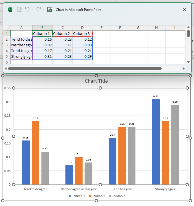
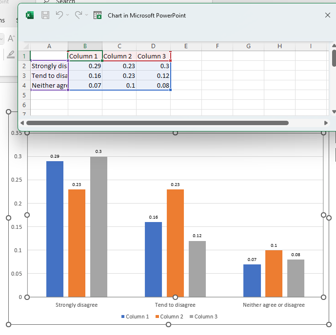
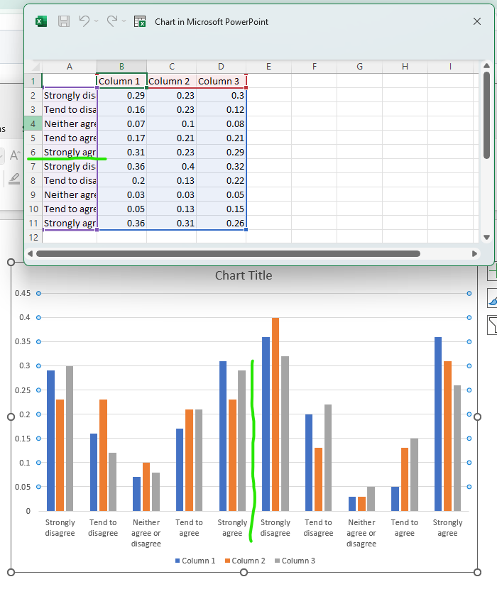
In the following example, we will be sorting our data in descending order based on the second column (the first column of data).

Files

Map the following query to the input template, which will grab our selected data and sort it:

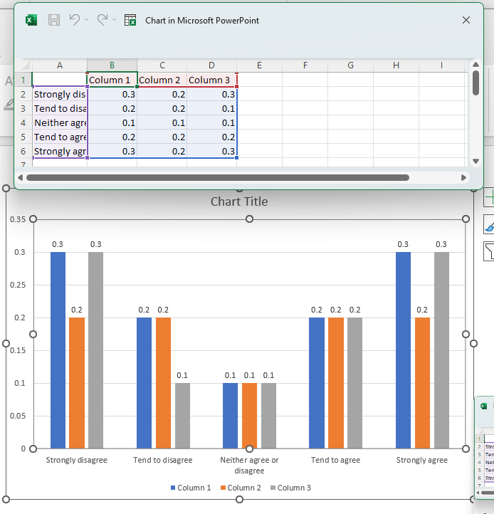
SELECT (f=1, t=1, r=[5:9], c=[1:4]) -> SORT_BY (by=[2], axis="rows", asc=False) >> (2, 1)

Selected data from the data file

tab image

Download the slide and you should get the following result:

tab image

Here we can see that Column 1 has been sorted in descending order, and the other columns have been moved alongside it.

FILTER

Filters out columns or rows from a specified range if the their values don't meet the condition.

Parameters:

Name	Type	Description	Default
`condition`	`Condition`	if a value meets the condition. the corresponding row/column will be filtered out.	required
`axis`	`Axis`	filter on rows (0) or columns (1).	`1`

Raises:

Type	Description
`TypeError`	when comparator >, >=, < or <= is used on non-numerical values.

Example

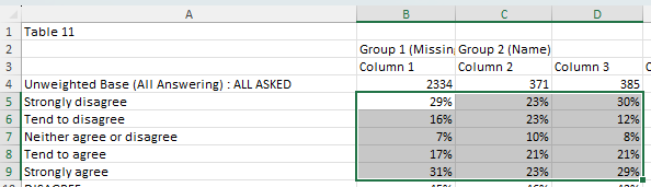
In the following example, we will be removing any row that contains the text "Strongly disagree" from our data selection.

Files

Map the following query to the input template, which grabs our selected data and applies the filter transformation.

SELECT (f=1, t=1, r=[3, 5:9], c=[1:4]) -> FILTER (condition = x == "Strongly disagree", axis="rows") >> (1, 1)

Selected data from the file with the row to be removed highlighted tab image

Download the slide and you should get the following result: tab image

The "Strongly disagree" row from the data file has been filtered out.

PIN

Pins a subset of rows/columns to the top or bottom.

Parameters:

Name	Type	Description	Default
`index`	`Index`	which rows/columns to move.	required
`axis`	`Axis`	pin rows (0) or columns (1).	`0`
`how`	`"top" \| "bottom"`	pin to top or bottom	`"top"`

Raises:

Type	Description
`IndexError`	when `index` is not present in the dataframe.

Usage

PIN(index=[1], axis=0, how="top")

or a short version with defaults:

PN([1])

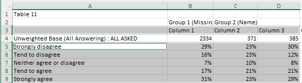
Example

In the following example, we will be pinning the "Neither agree or disagree" row to the top of the data selection.

Files

Map the following query to the input template, which will grab our selected data and move the specified row to the top.

SELECT (f=1, t=1, r=[5:9], c=[1:4]) -> PIN (index=["Neither agree or disagree"], axis="rows", how="top") >> (2, 1)

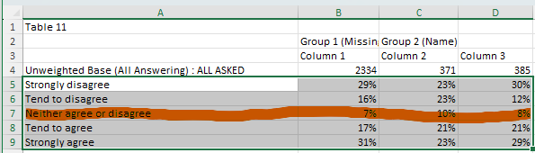
Selected data from the file, with the row to be pinned highlighted tab image

Download the slide and you should get the following result: tab image

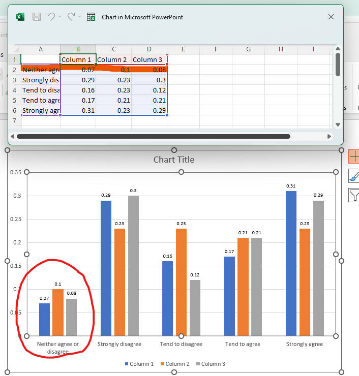
Here we can see that the "Neither agree or disagree" row has been pinned to the top of the data selection.

TRIM

Removes all but a specified subset of rows/columns.

Parameters:

Name	Type	Description	Default
`index`	`Index`	which rows/columns to preserve.	required
`axis`	`Axis`	apply to rows (0) or columns (1).	`0`

Raises:

Type	Description
`IndexError`	when `index` is not present in the dataframe.

Usage

Reduce dataframe to specific rows/columns

TRIM([1, 3, 4], "rows")
# also works with names
TRIM(["Column 1":"Column 5"], "columns")

Example

In the following example, we will be trimming the data so that only the first four rows remain.

Files

Map the following query to the input template. This contains the full selection of data as well as the TRIM transformation to keep just the first 4 rows (including the column labels).

SELECT (f=1, t=1, r=[3, 5:9], c=[1:4]) -> TRIM (index=[1:4], axis="rows") >> (1, 1)

Selected data from the data file tab image

Download the slide and you should get the following result: tab image

Here we can see that only first four rows of data are left from our original selection.

SUM

Gives the sum of the provided values.

Parameters:

Name	Type	Description	Default
`axis`	`Axis`	sum values over the axis. If not provided (default), returns the total of all values.	`None`
`numeric`	`boolean`	treat all values as numeric, otherwise raises an error when a non-numeric value occurs	`True`

Usage

# maps a single value to the specified cell
SUM(SELECT(...)) >> (2, 2)
# `axis=1` will give us a column that contains the sums of values in each row 
SUM(
    SELECT(...),
    axis="rows"
) >> (2, 2)

Example

Consider the following data source:

                                  0         1         2         3         4         5         6
1                                    Column 1  Column 2  Column 3  Column 4  Column 5  Column 6
2                             Row 1      8.57     43.85     14.28     66.72     43.67     17.64
3                             Row 2      6.25     62.11     87.85     92.13     54.42     55.83
4                             Row 3       8.5     26.15     22.12     55.24      91.9     54.68
5                             Row 4     40.16     26.83      0.27     71.47     14.35     97.91

Using SUM without specifying an axis:

SUM(SELECT(f=1, t=1, r=[1:5], c=[3, 4])) >> (1, 1)

yields the following result (the sum of all values in Column 3 and Column 4):

        0
0  283.46

If the axis argument is provided:

SUM(SELECT(f=1, t=1, r=[1:5], c=[3, 4]), axis="rows") >> (1, 1)

we get a data frame with an orientation that matches the axis value:

Note that the value in the first row evaluates to 0 because we have column names in that row. This behavior can be disabled by setting the numeric argument to False. In which case, an error will be thrown instead.

TRANSPOSE

Switches rows and columns.

Usage

It takes no arguments, so it's quite straightforward:

TRANSPOSE()

or

T()

Example

In the following example, we will perform a transpose action on our data selection.

Files

Map the following query to the input template:

SELECT (f=1, t=1, r=[3, 5:9], c=[1:4]) -> TRANSPOSE() >> (1, 1)

Selected data from the file tab image

Download the slide and you should get the following result: tab image

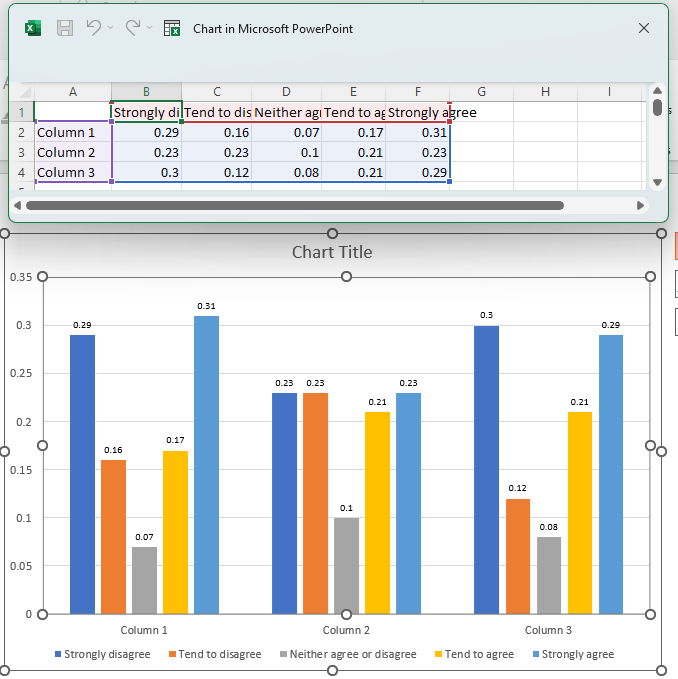
Here you can see that the columns and rows have been swapped.

FORK

Substitutes with value A if condition is true else with value B.

Parameters:

Name	Type	Description	Default
`condition`	`Condition`	a comparison expression.	required
`x`	`DataFrame`	yield value when condition is met.	required
`y`	`DataFrame`	yield value when condition is not met.	`""`

Raises:

Type	Description
`TypeError`	when comparator >, >=, < or <= is used on non-numerical values.

Usage

FORK(x > 100, "big", "small")

or a shorter version:

FK(x > 100, "big", "small")

Example

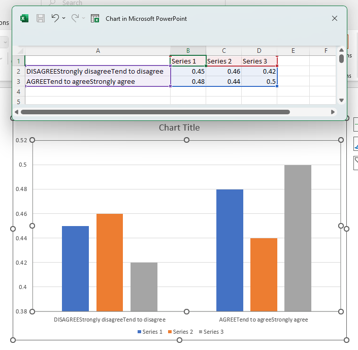
In the following example, we will be replace all the values in the selected range with "big" if they are greater than 0.20 and "small" if they are less than 0.20.

Files

Map the following query to the input template, which will select our data range and then apply our condition to it. This will check whether each value in our selection meets the condition, and apply the first option "big" if it does, or the second option "small" if it doesn't.

SELECT (f=1, t=1, r=[5:9], c=[2:4]) -> FORK (x > 0.20, "big", "small") >> (2, 2)

Download the slide and you should get the following result: tab image

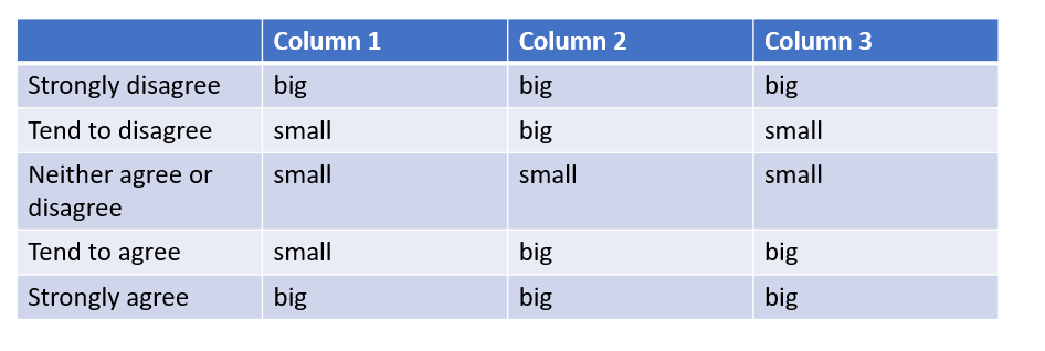
Here we can see all the number values have been replaced depending on whether or not they met the condition.

REPLACE

Finds and replaces values from the contextual data set with values from another data set.

Parameters:

Name	Type	Description	Default
`keys`	`DataFrame`	a dataset that contains values that need to be replaced.	required
`values`	`DataFrame`	a dataset that contains replace values.	required

Usage

REPLACE(
    SELECT (1, 1, [3:5], [1]),
    SELECT (2, 1, [1:3], [1])
)

Example

In the following example, we will be replacing the names of two row labels.

Files

Map the following query to the input template, which will grab our selected data and target the "Strongly disagree" and "Strongly agree" labels with the REPLACE transformation.

SELECT (f=1, t=1, r=[3, 5:9], c=[1:4]) -> REPLACE (["Strongly disagree", "Strongly agree"], ["Very negative", "Very positive"]) >> (1, 1)

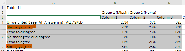
Selected data with the rows to replace highlighted tab image

Download the slide and you should get the following result: tab image

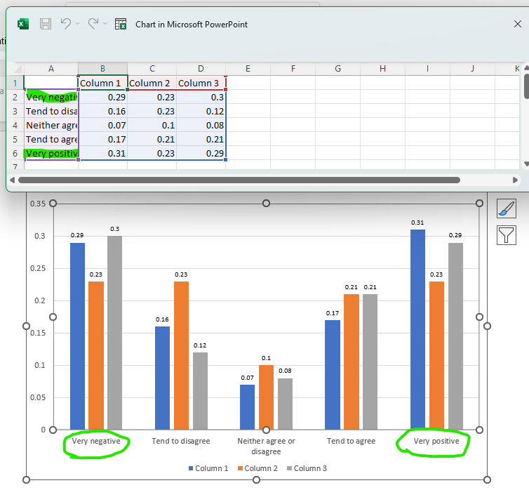
Here we can see that the two targeted rows have been renamed to "Very negative" and "Very positive" respectively.

FORMAT

Formats values to strings with optional prefix and suffix

Parameters:

Name	Type	Description	Default
`prefix`	`str`	prepend specified characters to the value.	`""`
`suffix`	`str`	append specified characters to the value.	`""`
`code`	`str`	Excel number format code.	`""`
`rows`	`Index`	apply formatting to specific rows only.	`[:]`
`columns`	`Index`	apply formatting to specific columns only.	`[:]`

Raises:

Type	Description
`ValueError`	when applying formatting code to a value that cannot be converted to a number.

Usage

FORMAT(prefix="=", suffix="%", rows=[1:5], columns=[2:4])

or a shorter version:

FT(px="=", sx="%", r=[1:5], c=[2:4])

Remarks

This transformation can also be used with no arguments to change data type to string.

The following format codes are supported:

#,###
#,
0
0.0
0.00
0.000
0,0
0,00
0,000
0%
0.0%
0.00%
0.000%
0,0%
0,00%
0,000%

Example

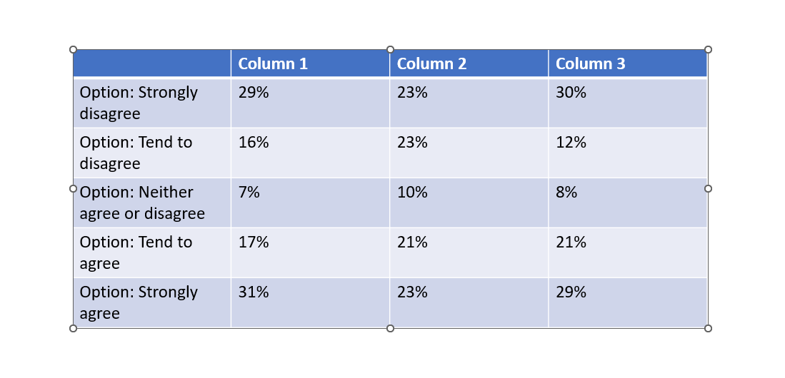
In the following example, we'll be adding the prefix "Option: " to each of the row labels, and reformatting the values to percentages by adding a "%" suffix to them.

Files

Map the following query to the template. This is composed of two parts, one to add the row labels and the other the data values. Each on has its own FORMAT transformation to apply the prefix and suffic respectively. For the 2nd query, we are also adding a multiplication and ROUND to better format the values. This is not part of the FORMAT transformation.

SELECT (f=1, t=1, r=[5:9], c=[1]) -> FORMAT (prefix="Option: ") >> (2, 1)
SELECT (f=1, t=1, r=[5:9], c=[2:4]) *100 -> ROUND() -> FORMAT (suffix="%") >> (2, 2)

Download the slide and you should get the following result: tab image

ROUND

Rounds values to a specified number of digits.

Parameters:

Name	Type	Description	Default
`ndigits`	`int`	the number of digits to which values should be rounded.	`0`

Raises:

Type	Description
`TypeError`	when attempting to round non-numeric values.

Usage

Round to 2 decimal places:

ROUND(2)

or a shorter version:

RD(2)

Remarks

If ndigits is greater than 0, then number is rounded to a specified number of decimal places.
If ndigits is 0, the number is rounded to the nearest integer.
If ndigits is less than 0, the number is rounded to the left of the decimal point.

Example

In the following example, we will round our data set to 1 decimal place.

Files

Map the following query to the input template, which will grab our selected data and perform the rounding.

SELECT (f=1, t=1, r=[5:9], c=[2:4]) -> ROUND(1) >> (2, 2)

Selected data from the data file tab image

Download the slide and you should get the following result: tab image

Normally, the decimal formatting from the data file will be converted to 2 decimal places by default. But since we have applied the ROUND transformation, all the values have been formatted to 1 decimal place.

INSERT_BLANK

Inserts arrays of a coherent shape with empty values (null) into the contextual data set.

Parameters:

Name	Type	Description	Default
`index`	`Index`	dictates where empty columns/rows shall be inserted.	required
`axis`	`Axis`	apply row (0) or column (1) wise.	`0`

Raises:

Type	Description
`IndexError`	when `index` is not present in the dataframe.

Usage

INSERT_BLANK([2, 4, 6], 0)

or a shorter version with defaults:

IB([2, 4, 6])

Remarks

Index values with step parameters might come especially handy here. For example, to insert a blank array after each column we can specify index=[1::1] (step over every 2nd starting after the first oneandaxis=1`.

Example

In the following example, we will be inserting a blank row on the 2nd, 4th and 6th row.

Files

Map the following query to the input template:

SELECT (f=1, t=1, r=[5:11], c=[1:4]) -> INSERT_BLANK (index=[2, 4, 6], axis="rows") >> (2, 1)

Selected data from the file tab image

Download the slide and you should get the following result: tab image

Here you can see that blank rows have been added after the 2nd, 4th and 6th rows from the original data selection.

This same result can be achieved by using a "step" index, specifying that a blank space should be inserted every two rows starting from the 2nd one and stopping at the 7th.

SELECT (f=1, t=1, r=[5:11], c=[1:4]) -> INSERT_BLANK (index=[2:7:2], axis="rows") >> (2, 1)

SIG_TEST

Picks up significance test results from the data source and renders them for the corresponding values.

Parameters:

Name	Type	Description	Default
`base`	`DataFrame`	comparison expression for base values
`sig`	`DataFrame`	comparison expression that determines significance of a value	required
`direction`	`DataFrame`	comparison expression that determines significance sign (+/-)	required
`formatting`	`tuple[str, str, str, str, str, int]`	See "Remarks" section

Usage

SIG_TEST(
    sig=SELECT(...) in SELECT(...) | SELECT(...) in SELECT(...),
    direction=SELECT(...) in SELECT(...)
)

A version with base and custom formatting options:

SIG_TEST(
    base=SELECT(...) > 100,
    sig=SELECT(...) in SELECT(...) | SELECT(...) in SELECT(...),
    direction=SELECT(...) in SELECT(...),
    formatting=["⬆", "green", "⬇", "red", "above", 13]
)

Remarks

The value of formatting argument defines visualisation of significance testing results. It must be an list of six values: positive symbol, positive color, negative symbol, negative color, symbol's position and symbol's font size. The default value is ["↑", "50,150,0", "↓", "200,0,0", "right", 13,]. The position argument must be one of these values: left, right, top, bottom

For more information, see the breakdown of how it works in the Recipies section.

Example

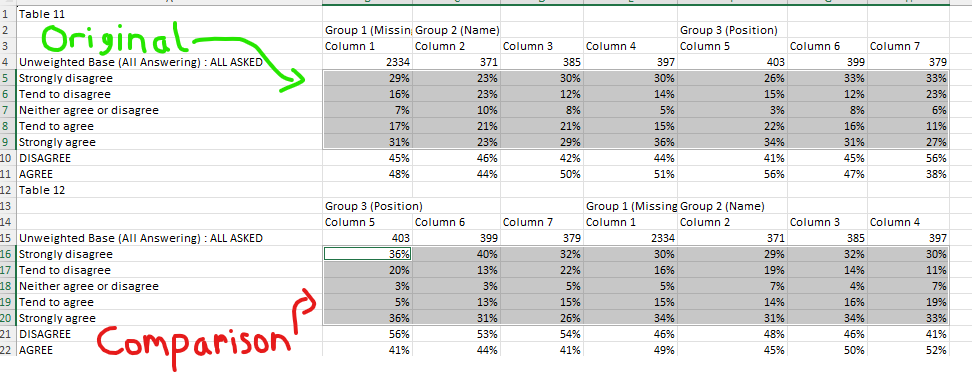
In the following example we'll be using signficance data in the below file to add significance arrows to the appropriate values.

tab image

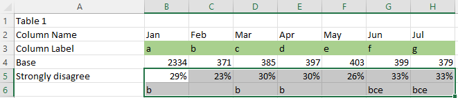
Here we'll be expecting an up arrow for the values at "Mar" and "Jun" and a down arrow at the value for "Feb", since they are significantly higher or signficantly lower than their previous columns.

Files

Map the following query to the table on the first slide of the input template.

SELECT (f=1, t=1, r=["Strongly disagree"], c=["Jan"]) -> ROUND(2) >> (2, 2)
SELECT (f=1, t=1, r=["Strongly disagree"], c=["Feb":"Jul"]) -> SIG_TEST (
    base=SELECT (f=1, t=1, r=["Base"], c=["Feb":"Jul"]) > 100,
    sig=SELECT (f=1, t=1, r=["Column Label"], c=["Jan":"Jun"]) in SELECT (f=1, t=1, r=["Strongly disagree"(+1)], c=["Feb":"Jul"])
    |
    SELECT (f=1, t=1, r=["Column Label"], c=["Feb":"Jul"]) in SELECT (f=1, t=1, r=["Strongly disagree"(+1)], c=["Jan":"Jun"]),
    direction=SELECT (f=1, t=1, r=["Column Label"], c=["Jan":"Jun"]) in SELECT (f=1, t=1, r=["Strongly disagree"(+1)], c=["Feb":"Jul"]),
    formatting=["⬆", "green", "⬇", "red", "right", 18])
-> ROUND(2)
>> (2, 3)

Download the slide and you should get the following result: tab image

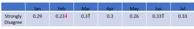
Here we can see that significance arrows have been added to the values we expected:

Feb received a down arrow because Jan has its significance letter (b), meaning that Feb is significantly lower
Mar received an up arrow because it has Feb's significance letter (b), meaning that Mar is significantly higher
Jun received an up arrow because it has May's significance letter (e), meaning that Jun is significantly higher

AUTO_SIG_TEST

Performs a significance test on a range of values from the ground up.

Parameters:

Name	Type	Description	Default
`other`	`DataFrame`	dataframe of comparative values.	required
`base`	`DataFrame`	base values for the contextual dataframe.	required
`base_other`	`DataFrame`	base values for the "other" dataframe.	required
`level`	`Float`	confidence level of the significance test	`0.95`
`rows`	`Index`	rows that need to be tested.	`[:]`
`columns`	`Index`	columns that need to be tested.	`[:]`
`formatting`	`tuple[str, str, str, str, str, int]`	See "Remarks" section

Raises:

Type	Description
`IndexError`	when `rows`/`columns` are not present in the dataframe.
`ValueError`	when the shape of the dataframe that is being tested doesn't match the shape of the "other" dataframe of comparative values.

Usage

SELECT(f=1, t=1, r=[2:4], c=[2:]) -> AUTO_SIG_TEST(
    other=SELECT(1, 2, [2:4], [2:]),
    base=SELECT(1, 1, [5], [2:]),
    base_other=SELECT(1, 2, [5], [2:]),
    level=0.95,
    rows=[:],
    columns=[:],
    formatting=["+", "green", "-", "red", "top", 11])
) >> (1, 1)

Remarks

The value of formatting argument defines visualisation of significance testing results. It must be an list of six values: positive symbol, positive color, negative symbol, negative color, symbol's position and symbol's font size. The default value is ["↑", "50,150,0", "↓", "200,0,0", "right", 13,]. The position argument must be one of these values: left, right, top, bottom

Example

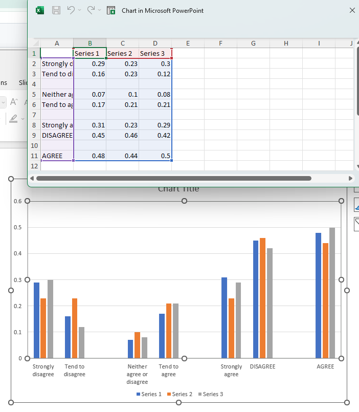
In the following example we will be comparing one table of data to another and having the plugin perform the sig test calculation itself.

tab image

Files

Map the following data to the input template:

SELECT (f=1, t=1, r=[5:9], c=[2:4]) -> AUTO_SIG_TEST (
other=SELECT (f=1, t=2, r=[5:9], c=[2:4]),
base=SELECT (f=1, t=1, r=[4], c=[2:4]),
base_other=SELECT (f=1, t=2, r=[4], c=[2:4]),
level=0.95,
formatting=["⬆", "green", "⬇", "red", "above", 13]
) >> (2, 2)

Download the slide and you should get the following result: tab image

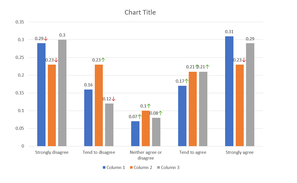
Here we can see values have been given an up or down arrow based on how much bigger or smaller they are than their respective values in the comparison data set.

REVERSE

Reverse the order of rows or columns in the dataset. Parameters:

Name	Type	Description	Default
`axis`	`Axis`	defines whether to reverse rows or columns	0

Usage

SELECT(...) -> REVERSE("columns")

LOWER

Convert to lower case.

Raises:

Type	Description
`TypeError`	when used on non-string values.

Usage

LOWER()

or a shorter version:

L()

Example

In the following example we will set all the row labels to lower case.

Files

Map the following query to the template, which performs two selections: the first on the row labels to be transformed, and the second to grab the data.

SELECT (f=1, t=1, r=[5:11], c=[1]) -> LOWER() >> (2, 1)
SELECT (f=1, t=1, r=[5:11], c=[2:4]) >> (2, 2)

Total selected data from the file across both queries tab image

Download the slide and you should get the following result: tab image

CONCAT

Concatenate multiple DataFrames and literals as strings.

Parameters:

Name	Type	Description	Default
`data_sources`	`list`	List of available data sources (unused but required by signature)	required
`*args`		DataFrames and/or literal values to concatenate	`()`
`**kwargs`		Additional keyword arguments (currently unused)	`{}`

Returns:

Type	Description
`DataFrame`	DataFrame with concatenated values

Example

In the following example, we will combine two sets of three column labels together to make two long column labels.

Files

Map the following query to the template, which performs two functions: the first combines the different column labels, and the second grabs the data.

CONCAT (
SELECT (f=1, t=1, r=[10, 11], c=[1]),
SELECT (f=1, t=1, r=[5, 8], c=[1]), 
SELECT (f=1, t=1, r=[6, 9], c=[1])
) >> (2, 1)

SELECT (f=1, t=1, r=[10, 11], c=[2:4]) >> (2, 2)

Selected data from the file tab image

Download the slide and you should get the following result: tab image

Here we can see that the selected row labels have been combined.

IIF

Conditionally select values based on boolean conditions (if-then-else logic).

Parameters:

Name	Type	Description	Default
`data_sources`	`list`	List of available data sources (unused but required by signature)	required
`bool_frame`		Boolean DataFrame or condition to evaluate	required
`a`		Value/DataFrame to select when condition is True	required
`b`		Value/DataFrame to select when condition is False (default: "")	`''`
`iterate`		Whether to iterate over individual boolean values. If False, uses .any() on the boolean frame. Defaults to True	`None`

Returns:

Type	Description
`DataFrame`	DataFrame with conditionally selected values

Example

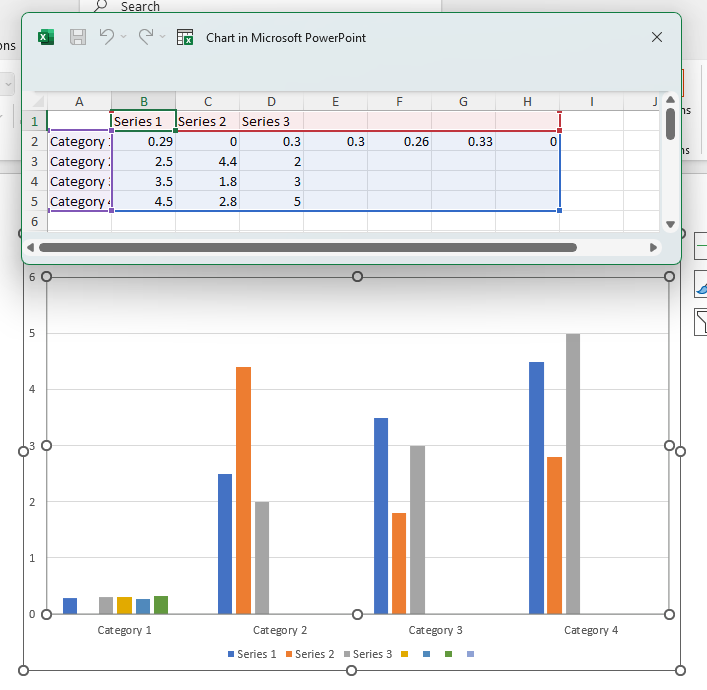
In the following example, we will apply a condition that will only retrieve a value from one row if the row above it contains a value greater than 380. If it's value is less than 380, 0 will be returned instead.

Files

Map the following query to the template, which will apply the IFF condition to the selected data.

IIF (
SELECT (f=1, t=1, r=[4], c=[2:8]) > 380,
SELECT (f=1, t=1, r=[5], c=[2:8]),
0
) >> (2, 2)

Selected data from the file tab image

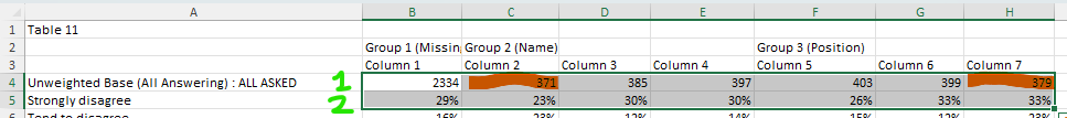
Here we expect the values in column C and 7 to return 0, rather than their respective values in the second row, since their values in their first row do not meet the condition.

Download the slide and you should get the below result: tab image

JOIN

Join a sequence of DataFrames along an axis.

Combines multiple DataFrames or lists by concatenating them along the specified axis. Handles significance testing results by preserving and merging sig settings.

Parameters:

Name	Type	Description	Default
`data_sources`	`list`	List of available data sources (unused but required by signature)	required
`*args`		DataFrames or lists to join	`()`
`**kwargs`		Keyword arguments including: axis: Axis to join along (0 for rows, 1 for columns). Defaults to 0	`{}`

Returns:

Type	Description
`DataFrame`	DataFrame with joined data, including MultiIndex columns if any input has sig testing

Usage

JOIN(
    SELECT(1, 2, [4:8], [2:5]),
    SELECT(1, 4, [5, 6], [2:5]),
    axis=0
)

Remarks

Normally, when joining DataFrames by row (column) axis, they should have the same amount of columns (rows). However, if they don't, it won't raise an error. Instead, the "missing" columns (rows) will be filled with null values.

Example

In the following example, we will combine two data sets from different tables and stack them on top of each other (by rows).

Files

Map the following query to the input template, which grabs our two data sets from different tables and designates how they should be combined.

JOIN (
SELECT (f=1, t=1, r=[3, 5:9], c=[1:4]),
SELECT (f=1, t=2, r=[5:9], c=[1:4]),
axis="rows"
) >> (1, 1)

Selected data from the file tab image

Download the slide and you should get the following result: tab image

Here the divide between the two sets of data has been highlighted to demonstrate how they have been combined.

UPLOAD

Split data files to be read by the plugin.

Parameters:

Name	Type	Description	Default
`name`	`str`	name of the data source.	`"main"`
`pattern`	`str`	a cell that matches this argument's value will identify the row by which the data source should be splitted into multiple tables.	`""`
`column`	`int`	the values of the specified column will be matched against the pattern.	`1`
`sheet`	`int`	the sheets from the data source that should be used.	`1`
`name_loc`	`tuple[int, int]`	coords of the cell containing the table name.	`None`
`offset`	`int`	offsets rows matching the pattern when splitting tables.	`0`
`banner`	`tuple[int, int]`	the start and end rows that comprise a banner. If specified, the banner will be prepended to each table in the sheet. If a banner is comprised of a single row, the start and end must have the same value, e.g. `[1, 1]`.	`None`

Example

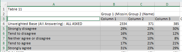
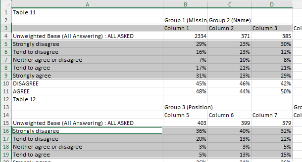
In the following example, we'll be splitting a simple file into tables and identifying where each table name can be found.

Files

In the "Connect data" table, click "Choose File" and upload the Training data file. Add the following query to the text field:

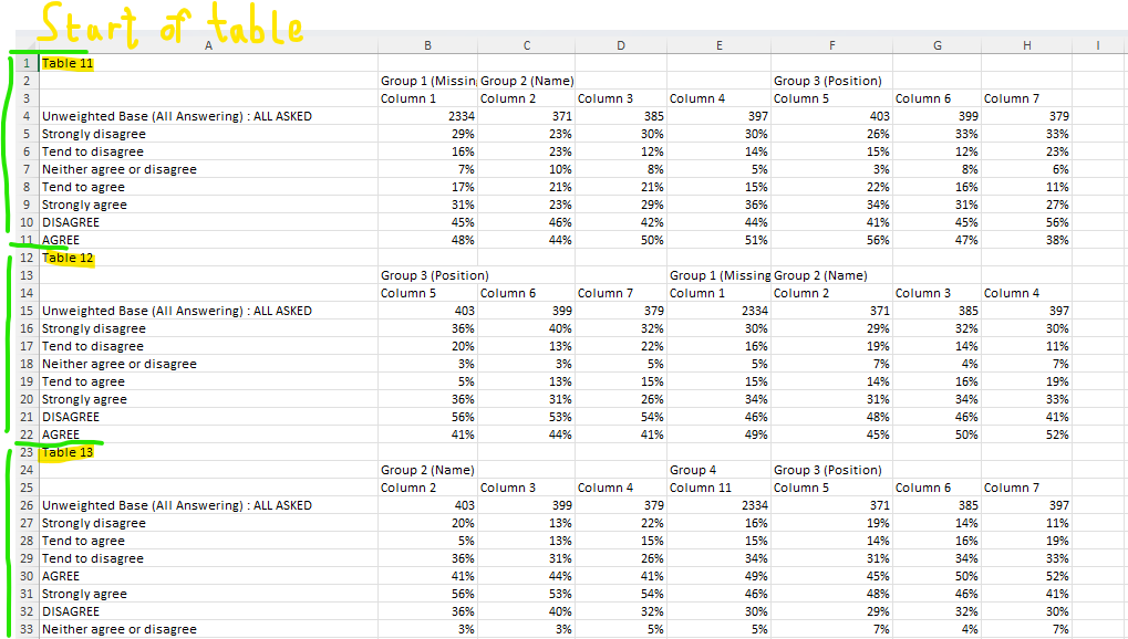
UPLOAD (name="training", pattern="Table\s\d+", column=1, sheet=[1,2], name_loc=[1, 1])

This UPLOAD query identifies where the start of each table is using its pattern argument. Using python regular expressions, it determines that the first table should start at Table 11, the second at Table 12, and so on. You can learn more about python regular expressions here. ChatGPT is also good at writing these.

It knows to look in the first column for these strings because of our column argument. We have specified sheet=[1, 2] for this query, which means we can use either of the first two sheets for our SELECT queries.

It will include the first and second sheets of the file in the upload. Both sheets will be split according to the other arguments.

Finally, we have indicated that the name of each table can be found in its first row and first column. Since Table 11, Table 12, etc. are identified as the first cell in each table, the plugin will treat these as the table names.

tab image